Picking a cloud database for analytics: the SQL options
If you’re a developer, analyst, or data scientist, you have probably been hearing a lot about “analytics” these days. Some the most popular open source big data projects, like — Spark, Cassandra, and Elasticsearch — regularly tout their analytics abilities. But it’s only in the last 18 months that good old SQL has re-emerged as a formidable analytics technology.
What’s going on? I thought “NoSQL” was for analytics data, and SQL was for business data?
Well, we’re going to unpack that all today. In particular, we will discuss how SQL is used for analytics, and how analytics queries are supported by real-world cloud SQL services.
This post started with a tweet:

… and, keeping the promise of that tweet — and the many replies and likes it received — this post will compare:
It will also serve as a guide for choosing between these options, including the technical pro’s and con’s of each.
How SQL is used for analytics
SQL — the language, the concept — actually excels at analytics.
What is analytics, from a technical point-of-view? It’s really two interlocking functions over your data: reporting and analysis.
Reporting answers the “how many?” question, and typically involves these three query components:
- aggregating some data
- over some time period
- with some filtering applied
For example, the classic reporting query is, “how many hits did my website get in the last 7 days?” This could be expressed as a SQL query like the following:
SELECT COUNT(action) as views
FROM parsely.rawdata
WHERE
action = 'pageview' AND
ts_action > current_date - interval '7d';
(Here, we’re using Postgres dialect of SQL.)
The SQL table is assumed to contain one row per event, with action = 'pageview' indicating a pageview event, and where ts_action is the timestamp of the event. The aggregation, COUNT(...), is a simple count of all of those events. SQL has several common aggregates supported in the standard, including COUNT, SUM, MAX, COUNT(DISTINCT ...), etc.
Analysis is about drawing some conclusion from your data. Rather than answering the “how many?” question, we aim to answer the “why?” question.
For example, let’s say you determine that in the last 7 days you saw a spike in page views on your site, which you determined via one of th above reports.
You might wonder, “Yes, but why did traffic spike?” So then you may try to characterize everything you know about this week. For example, this SQL query could select all the data from this week, and break out all the traffic sources by referrer domain and the URL of the pageview.
SELECT ref_domain as domain, url_clean as url, COUNT(action) as views
FROM parsely.rawdata
WHERE
action = 'pageview' AND
ts_action > current_date - interval '7d'
GROUP BY 1, 2
ORDER BY 1;
Now we’re digging into the spike and finding the domain and url that received the most clicks on that day, so we can try to understand it a little better. This is a simple query, but it starts to get into analysis — answering the “why?” questions around our sites and apps.
As you can see, SQL does well at both of these core analytics tasks: reporting and analysis.
Why not SQL engines for analytics?
So, if the SQL language is good at this stuff, why haven’t people been using SQL engines for analytics? In a word: performance.
The only reason SQL has not been the obvious first choice for analytics in the last few years is due to machine and data limitations of most common single-node SQL engines, specifically the typical Postgres and MySQL database setups you find powering the lion’s share of modern applications.
For example, if you install Postgres on a server, you will be limited by CPU, memory, disk, or all three.
Let’s say you have a 100 GiB disk for this database server. Well, you can only store a little less than 100 GiB of total data. Some websites have so much traffic that raw page view events would fill up a 100GiB disk pretty quickly — perhaps in a few days. So, that’s the disk limitation.
NoSQL stores solve disk limitations with horizontal data sharding strategies, such as the consistent sharding strategy famously used in Cassandra.
What about CPU or memory? Well, let’s take one of the most painful kinds of analytics for many SQL databases: COUNT(DISTINCT ...). If you have ten million page view events, and you want to count unique visitors across those events, you might need to write a SQL query like this:
SELECT COUNT(DISTINCT visitor_site_id)
FROM parsely.rawdata
WHERE
action = 'pageview' AND
ts_action > current_date - interval '7d';
On Postgres and MySQL, the performance of this query will be quite atrocious if the number of page view events is high.
In each database, an in-memory set of the unique identifiers will need to be constructed by the database engine, and a full table scan will be performed. Even if your CPU keeps up with the scan, your memory probably won’t keep up with the cardinality of that set. If the disk of this server is 100 GiB, your memory is bound to be a fraction of that, like 16 GiB, so this query will simply fail — and perhaps even crash your server.
Open source technologies like Elasticsearch and Spark work around this problem by using multi-node parallelism, thus agglomerating CPU and memory from a cluster of machines. They also use approximation algorithms, known as “data sketches”, to achieve acceptable performance for the particularly problematic “count distinct” problem. But to do so, they end up moving outside of traditional SQL capabilities.
Single-Node vs Multi-Node
Traditionally, SQL engines are single-node. Thus, the only way to scale them is to get a bigger machine. One thing that NoSQL engines do well is multi-node, or cluster, operation.
In the case of a system like Cassandra, multi-node means that data can spread evenly across nodes, avoiding the limits of a single disk. In the case of systems like Spark and Elasticsearch, memory and CPU is spread across multiple nodes, as are the “working sets” of data and computation (such as aggregations).
So, when you run a query similar to the queries above, they “scatter-gather” across the cluster to speed up the query and use cluster-wide resources.

Memory vs SSD vs Spinning Rust
Traditionally, SQL engines run on machines with relatively little memory and large “spinning rust” disks. Because the database knows that memory is limited and disk access is expensive (from a performance standpoint), the database tries to use a fixed amount of RAM and speed up disk access using indices.
But in the case of modern cloud computing hardware and data centers, gobs of system memory have become cheaper, and SSDs have all but replaced spinning rust in standard deployments. Due to this, it can be faster to load large working sets of data into memory, or lay them out efficiently on SSDs, to provide interactive query speeds.
Row-Wise vs Column-Wise
A big difference between standard SQL engines, like MySQL and Postgres, and the new crop of NoSQL engines, like Elasticsearch and Cassandra, is what is known as row vs columnar storage.
To illustrate this difference, consider our millions of page views. Imagine if one database stored the millions of page views like this:
row1 = {"url": "/article1", "views": 1, "starts": 0}
row2 = {"url": "/article2", "views": 1, "starts": 0}
row3 = {"url": "/article2", "views": 0, "starts": 1}
row4 = {"url": "/article1", "views": 1, "starts": 0}
save("events.db", [row1, row2, row3, row4])
Whereas the other database stored them like this:
column1 = ["/article1", "/article2", "/article2", "/article1"]
column2 = [1, 1, 0, 1]
column3 = [0, 0, 1, 0]
save("column1.db", column1)
save("column2.db", column2)
save("column3.db", column3)
Now let’s imagine both databases have to store the entire “table” on-disk, and the format chosen is as follows. For the first database, 1 file, events.db, is stored. The file consists of 4 lines, with each row in row1..4 on each line. For the second database, 3 files are stored, named column1.db, column2.db, column3.db, and these store the data in each column in column1..3, each as separate lines.
To query either database, you need to load parts or all of the data into memory. But there’s a question of how much work you have to do to get the relevant data. If there millions of such events, the second database design — the column-oriented one — will have a much easier time counting the views.
Why is that? Well: it can just slurp that array of view integers, represented there by column2 and stored in column2.db, directly into memory, and calculate a fast SUM. The row-based database would need to load, parse, and scan all rows to count the views. This is the essential difference between column- and row-oriented storage.
Rob Story, in his presentation on Simple’s use of a Redshift SQL Warehouse, describes this distinction quite well in this slide:

Obviously, column-oriented storage has some downsides. For example, if you modify or delete a “row” of data, you need to update N database files — one for each column in your database table. This can be make UPDATE and DELETE operations very slow. But column-oriented storage has so many extra benefits for query time. Column-oriented database systems can compress data more easily, filter data more quickly, and scan data more efficiently — all thanks to the column-stride format.
NoSQL is cool, but I love SQL!
Given the above advantages of NoSQL systems, are you doomed to use them instead of SQL forever? Do you now need to puzzle over their odd query languages and beg your devops staff to spin you up expensive clusters?
Nope! The cloud has the answer. And the answer is, unsurprisingly, a “hybrid approach”. The convenience of the SQL language and interface, mixed with the power of cloud and cluster computing. Enter: the cloud SQL engines.
Cloud Postgres and MySQL

Amazon and Google recognize that a major part of any data center footprint involves regular SQL databases. They further know that the widespread success of the largest open source SQL communities — MySQL and Postgres — create network effects that are unbeatable.
As a result, it is no surprise that Amazon and Google each offer a “fully-managed” experience around these open source projects; let’s now dive into how these systems might work with analytics data.
Amazon RDS
Amazon’s Relational Database Service (RDS) is an established offering from AWS to run PostgreSQL in the cloud.
In their words, “you can deploy scalable PostgreSQL deployments in minutes with cost-efficient and resizable hardware capacity.” Sounds promising. So, what’s going on here?
RDS is not that different from running your own stock PostgreSQL engine. The key benefit is that you can elastically expand compute, disk, and memory via the Amazon control panel and APIs.
It does not provide any magic answer for the COUNT DISTINCT problem. That will still be slow on many events. But instead of being stuck with whatever server you pick up-front for your database, RDS lets you start with a small database with a slow disk, and pay more money for a bigger database with a bigger and faster disk. This can be helpful as you start to ingest more and more analytics-style event records into the DB.
You also get read replicas for free, which can be important for analytics use cases. By separating your read and write path, you’ll ensure your expensive analytics queries are not slowing down your database such that it can’t keep up with new data as it arrives.
For small scale use cases, RDS works perfectly fine, and benefits from lots of simplicity. Specifically:
- since it’s “just Postgres”, it works with all your existing drivers and tools
- since it’s “just SQL”, you can use all the filtering, subselect, and aggregation tricks you’re used to with a SQL engine
- since it’s hosted by AWS, you don’t have to worry about resizing clusters when you run out of space; this is something AWS can do with a few clicks
- since it’s hosted by AWS, you can set up read replicas that are dedicated “analytics query nodes” used solely by your analyst teams

One of the sore spots for using a tool like Postgres and RDS for analytics is its poor support for unstructured data that is common in analytics use cases. For example, if you have a “big pile of JSON” events, you’ll need to write your own tools to translate those into SQL INSERT statements, and you’ll need to be careful how you batch load those queries into your database. But, again, at small scale, this might not be a big deal.
Google Cloud SQL
Google’s Cloud SQL offering, which just exited beta, is similar to RDS, but in Google’s public cloud. It only runs on MySQL.
(Note: I know that Amazon RDS also supports MySQL, and even has a ‘special’ MySQL offering called Aurora. But for the purposes of this post and my own sanity, I’m going to avoid wading into those weeds.)

Similar to RDS, Google’s offering is fully-managed. They handle backups, replication, updates, etc. Just as with Postgres, you’ll find analytics queries will be limited to disk, CPU, and memory at certain scale. But at least you’ll be able to use Google’s snazzy control panel to resize your database nodes or setup replicas with zero ops work and minimal downtime.
Analytics Engines on Cloud Clusters

Parallel Cloud Analytics Engines like Amazon Redshift and Google BigQuery are very different from the above two products. Rather than offering a hosted version of an open source SQL engine, these services offer fully-managed multi-node (cluster) for doing analytics, but targeted at SQL analysts. In each case, the underlying technology is not open source; they are proprietary analytics engines that offer varying degrees of SQL support.
So, in addition to being contrasted from the hosted SQL options above, they should also be contrasted from open source analytics engines, like Elastic, Presto, Spark, and Druid. Each of these systems is fully open source, like MySQL and Postgres are. You can run them on your own local development boxes, and on your own clusters and machines, in any cloud. That does mean you have to master them from both an operational and query language standpoint. Elastic and Druid have specialized query languages and data models, whereas Spark and Presto have limited SQL implementations.
Amazon Redshift and Google BigQuery can be viewed, from this vantage point, as offering hosted, proprietary approaches to cluster analytics. The carrot is an ease of data loading and querying, in some cases with full SQL compatibility; the stick is vendor lock-in.
Further, as was shown in this small poll I did on Twitter, Amazon and Google run the market-leading technologies in this category.

Some other players exist, such as Snowflake’s cloud SQL warehouse and NewRelic’s SQL-flavored analytics engine that powers their “NewRelic Insights” product, but the truth is, I don’t see these coming up too often in the consideration set of practitioners in the field.
These days, CTO’s and VP’s of Data/Analytics, as well as product/data leads on small technical teams, are viewing the build vs buy decision as a battle of Spark / Hadoop / Elastic / et al for open source self-hosted options vs Amazon Redshift / Google BigQuery for proprietary hosted options, and sometimes they are even adopting “all of the above” for different products/apps within their business.
Amazon Redshift
Alright — so, RDS and Cloud SQL are fully-managed, but mainly single-node, SQL engines. They aren’t really “made for analytics”, but they can be used for analytics as long as you don’t hit the scaling limits.
Redshift is something else altogether. It’s very, very different.
Even though Redshift also runs in AWS and also offers a Postgres-flavored SQL interface, it is not your typical SQL engine.
Similar to RDS, Redshift is fully-managed. A few clicks in your AWS dashboard and you have a Redshift instance up-and-running. But unlike RDS, Redshift is not limited to single machines. Every Redshift database is actually a cluster of machines.
And, unlike an RDS-powered Postgres instance, data stored in Redshift uses “columnar storage technology to improve I/O efficiency and parallelizing queries across multiple nodes.”

Here’s a snippet from the best part of Redshift’s marketing material:
“Redshift uses columnar storage, data compression, and zone maps to reduce the amount of I/O needed to perform queries.”
Let’s break that down. Columnar storage means that when you load homogenous, structured data into a Redshift table, your aggregates can run per-column, rather than requiring full table-and-row scans. This saves a whole lot of CPU time and disk I/O.
Data compression — using Redshift schema extensions, you can have it compress data in the columns of your table that you expect to be repeated. This will trade a little CPU for decompression for a whole lot less disk I/O, which is usually a good trade.
Zone maps — this is an optimization for data that has a “typical” ordering. For example, time series data may be stored in Redshift in time order. To quote Amazon’s documentation, “When you sort a table, we use zone maps (cached in memory) to skip 1 MB blocks without relevant data. […] If a table has five years of data sorted by date, 98% of the blocks can be eliminated when you query for a particular month.”
Let’s continue to break down the marketing language, and interpret it for our pageview example:
“Amazon Redshift has a massively parallel processing (MPP) data warehouse architecture, parallelizing and distributing SQL operations to take advantage of all available resources. The underlying hardware is designed for high performance data processing, using local attached storage to maximize throughput between the CPUs and drives, and a 10GigE mesh network to maximize throughput between nodes.”
Ah hah. So, after all the above optimizations, you’ll still have to scan/count/sum something. But, Redshift lets you achieve strong performance even when it finally makes CPU your analytics bottleneck, through the classic techniques of parallel compute. It’ll have your data sharded on several Redshift “nodes”, and each of those nodes will do a subset of the aggregation in map/reduce style. Thanks to fast internal network, the scatter-gather will be faster than waiting for the single node.
Now, to give you all these awesome features, Redshift has to make some tradeoffs. For example, Redshift is not meant to be used for lots of random INSERT statements, and especially not for random UPDATE or DELETE statements. For these use cases, RDS will perform more predictably. Redshift performs best if your table is like an “append-only log”.
In fact, Redshift warns you against using INSERT statements altogether, instead pointing you toward their excellent COPY command, which can bulk copy data from S3. A newer product from AWS called Kinesis Firehose allows you to use the Kinesis streaming write API to collect events, and it will automatically batch your events into S3 files and bulk load them using the Redshift COPY command. These are the “right ways” to ingest data into Redshift.

If that sounds a little onerous, consider this: most of the time, data analysts get heaps of JSON or CSV data, and need to “dump it” somewhere to run queries. Well, Redshift’s COPY command is specifically optimized for this kind of bulk loading use case. Indeed, the command will even do things like automatically parsing JSON-line formats, automatically decompressing gzip-compressed files in S3, and automatically parsing string-based embedded data types like timestamps.
How about that COUNT DISTINCT aggregate we discussed before? Oh yea, Redshift handles that, too. Their COUNT function adds an extension called COUNT APPROXIMATE DISTINCT, which “uses a HyperLogLog algorithm to approximate the number of distinct non-NULL values in a column or expression; queries that use the APPROXIMATE keyword execute much faster, with a low relative error of around 2%.” Pretty cool.
Hopefully, with these explanations, you can see that Redshift appears as a kind of analytics chimera. Yes, it has a SQL interface, which can plug into existing code and tools that need to run analytical queries. But it’s not like your typical SQL engine. It is restrictive on the write path, and extends SQL in certain ways, while attacking the core performance problems that made old SQL engines a poor fit for large-scale analytics. And all while offering the convenience of Amazon’s public cloud and relatively ops-free control panels.
Google BigQuery
“But why bother worrying about machines and clusters at all?”
This is probably the question the Google team posed when thinking through their own take on SQL-style analytics.

BigQuery is Google’s answer to Redshift, although its architecture is dramatically different. Some parts are the same: for example, to attack the core performance problems, BigQuery also uses columnar storage, compression, fast internal network, and multi-node data sharding.
But unlike Redshift, you don’t run “a BigQuery cluster”. Instead, you just get a BigQuery account, and with that account, you are given API access to a single, massive BigQuery cluster that is run by Google. It’s truly “SQL analytics as a service”, and it’s truly “zero ops”.
Similar to the Redshift COPY command, BigQuery provides a tool called bq that assists with bulk loading of JSON or CSV data. It can even sync that data from Amazon S3 buckets.
Intriguingly, BigQuery doesn’t shy away from the real-time streaming write problem. For a price, you can send BigQuery streaming writes via a publicly-documented HTTP API, where bulk inserts can happen in a streaming fashion. This API is wrapped up in official clients for Python, JavaScript, and other languages. You never send BigQuery an INSERT or UPDATE statement; you either send it streaming writes, or you bulk load data using the bq tool.
Up until a few months ago, the big difference between Redshift and BigQuery from a usability standpoint was that Redshift supported a SQL dialect that was very close to Postgres, and indeed was mostly compatible with standard Postgres clients. But BigQuery had its own quirky not-quite-SQL-but-sorta-SQL dialect. Most tools couldn’t work with it out of the box, so you had to use special client libraries or buy special connectors for your client tools.
But a couple months ago, their Standard SQL dialect went into beta. This means that BigQuery is much more directly comparable to Redshift on the client side. This also means that BigQuery will magically start working with BI tools that use standard connectors like JDBC and ODBC and expect to use “standard” SQL SELECT statements.
The truly amazing thing about BigQuery is just how fast it is on big data sets. Because every query can run on hundreds or thousands of partially-idle nodes in Google’s data center, pretty much every BigQuery analytics request will return in seconds, even when it’s doing a full scan of terabytes upon terabytes of data. To illustrate this power, Google has even published a number of public data sets, including the full set of all Wikipedia edits and the full set of Github commits, each of which is beyond terabyte scale.

Making BigQuery fast is not some grand data modeling or performance tuning exercise. It doesn’t require lots of expertise in setting up schemas or thinking through data distribution, sort keys, and the like. Instead, you just dump your data into BigQuery. If you can query it, then you can also query it quickly. It’s hard to come up with queries that “break” the system. Yes, some queries are faster than others, but no query is a showstopper for your database. Even if you manage to send it a really terrible query — for example, by abusing sub-selects and joins to create a cardinality explosion — your only punishment will be that the query aborts after a timeout period. You didn’t just “hose your database” — since Google runs a global BigQuery cluster for everyone, they’ve already got safeguards in place to make sure no one ruins it for everyone.
That peace of mind is certainly worth something.
SQL is back!
I’m a big fan of the NoSQL movement. It got the open source community thinking through different ways to solve the challenges of data distribution and parallel queries, in an era where data volumes grew at an alarming rate and vectors for database performance changed dramatically.
However, I’m sure the data analysts and data scientists who thought to themselves — “I just want to be able to query my data!” — felt quite hamstrung by having to learn the query languages of MongoDB, Elasticsearch, Cassandra, and other similar tools. These tools are good for developers to build amazing web products, but not so good for analysts to do analytical queries. SQL, the language, is really the perfect fit for that sort of thing.
I would know: my team at Parse.ly runs a massive analytics cluster atop Elasticsearch for our real-time analytics dashboard & API for publishers. But it was the recent excitement around cloud SQL engines that led us to also offer our backend data collection infrastructure as a service via Parse.ly Data Pipeline. What are the two most popular use cases for our Data Pipeline?
- to bulk load data into a Redshift cluster for full SQL over our analytics events
- to stream real-time data to BigQuery for a fully-managed real-time SQL layer

The other thing driving interest in cloud SQL engines is the rise of SaaS BI tools, such as Looker, Periscope, and Mode. These allow teams to “roll their own dashboard” atop these options, and this is especially attractive to data analyst teams who might have felt that they could do complex analysis, but without visualizations of those analyses, they couldn’t be acted upon by the business- and customer-facing teams.

So, this is happening: and we know, because we’re increasingly becoming a data source for SQL-fluent teams that are hosting their own warehouses.
Recap
Let’s recap quickly. Amazon RDS and Google Cloud SQL can let any analyst spin up a small Postgres or MySQL database for running analytics queries, and then scale it up when they need more CPU, disk, or memory. This can be done for low cost and with full compatibility with the “SQL of old”.
Amazon Redshift and Google BigQuery provide particularly compelling answers for running analytics queries on event data. Redshift lets you spin up a parallel cluster that will let you run unlimited queries at a fixed monthly or annual cost. BigQuery lets you get out of the cluster-running business altogether, and run any number of queries at a variable cost per query. And both offer ways to bulk load and stream in your raw data.
BigQuery is perhaps the most fascinating development in this space, because of the “no ops” and “no servers” approach. It’s a magic Google black box where you can dump terabytes of data, run queries that scan those terabytes of data, and get back answers within seconds.
As Felipe Hoffa, a BigQuery Developer Advocate, describes on this Reddit thread, BigQuery takes a lot of the deep thought and up-front architectural design you’d have to put into designing a SQL analytics warehouse, and boils it down to, “who cares — just dump your data and BigQuery will figure it out.”
That’s pretty much the definition of “commodification of big data”, and I suppose it’s no surprise that Google is the one to figure it out. With BigQuery’s new “standard SQL” beta, I suspect competition in this space won’t slow down, and we’ll continue to see some amazing innovation over the next few years.
Conclusion
As for me, I’m betting that with 50 billion web analytics events per month and counting, Parse.ly’s data set will be one of the most fascinating ones that people analyze using these new tools.
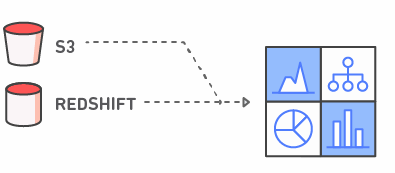
In fact, we’ve designed a reference architecture around Parse.ly’s Data Pipeline that allows us to use all sorts of analytical databases with our raw data. You can see a diagram of that architecture here:

More details can be found in our Data Pipeline technical documentation. If you have any questions — reach out to me via @amontalenti on Twitter.
—
Andrew is the co-founder and CTO of Parse.ly, a leading web/mobile analytics provider whose mission is to democratize data across organizations. His team’s work with the media industry includes powering the real-time dashboards used by staff at The Huffington Post, The Telegraph, Slate, Mashable, and many other top sites. The Data Pipeline powering Parse.ly’s suite of products operates at massive scale — and is now available as a fully managed service that anyone can license for their company or team. Andrew is also a dedicated Pythonista, JavaScript hacker, and open source advocate in the areas of Kafka- and Storm-based stream processing technologies. You can find Parse.ly on Twitter at @Parsely, and Andrew over at @amontalenti.
—
Appendix: Comparison Tables
I’ve put together a couple of tables comparing the various services on both features/approaches and on price. I’ve included them below.
Feature Comparison
| Service | Storage Limits | Sharding | Analytics Speedups | “Serverless” |
|---|---|---|---|---|
| Amazon S3 | None | N/A | No1 | Yes |
| Amazon RDS | 6 TB | No | No | No |
| Google Cloud SQL | 10 TB | No | No | No |
| Amazon Redshift | Petabytes+ | Yes | Sketches, Compression | No |
| Google BigQuery | Petabytes+ | Yes | Sketches, Compression | Yes |
- One of these is not like the other; S3 is obviously not a SQL engine. But it’s shown here to indicate why it tends to be involved in analytics discussions. S3 is a serverless way to just “dump your raw data”, and guarantee it’s durable and accessible.
Price Comparison
This table is not really a fair “apples and apples” price comparison, but more to show you the menu of options from a pricing standpoint, and to showcase the different pricing models. Note also that these prices do not include any discounts provided by up-front payment or commitment.
RDS and CloudSQL have low entry points: you can spend as little as ~$20-$100/mo to get started with single-node setups, and you’ll still have unlimited querying capability for playing around with small and large data sets. The costs of these, even for single-node setups, can go up to a few thousand dollars per month; the case of RDS, a massive node with 244 GiB of RAM will cost you around $2.8k/month for compute.
Redshift has a steeper starting price: the smallest one-node cluster will cost you $180/month, and typical clusters will probably be in the $500-$1,000/month range. But if you use reserved instances judiciously, you can achieve price points near a couple thousand dollars per year to have a TB or more of fast-queryable data.
BigQuery’s pricing model is just totally different than the others. It’s $20/mo per TB of data stored, and then $5 per TB of data queried. That means if you have a query that scans a full terabyte of data, that single query will cost you $5. But, you don’t have to pay a dime for unused compute capacity.
So, with all that said, here’s the summary:
| Service | Storage Cost | Compute Cost | RAM per Node |
|---|---|---|---|
| Amazon S3 | $30 per TB / mo | N/A1 | N/A1 |
| Amazon RDS | $115 per TB of SSD / mo | $13 – $2,865 per node / mo | 1 GiB – 244 GiB |
| Google Cloud SQL | $170 per TB of SSD / mo | $8 – $2,016 per node / mo | 0.6 GiB – 104 GiB |
| Amazon Redshift | N/A2 | $180 – $3,456 per node / mo | 14 GiB – 244 GiB |
| Google BigQuery | $20 per TB / mo | $5 per TB query3 | N/A3 |
- S3 has no notion of “node”, therefore no compute or RAM; S3 cost is provided as a baseline of “cheap cloud storage”.
- Redshift storage cost is tied to compute cost; there are options for regular disks and SSDs into terabyte ranges.
- BigQuery has no variable per-node compute costs or per-node RAM limits because its pricing model is based on the amount of data scanned per query in the BigQuery cluster.